import h5py
import matplotlib.cm as cm
import matplotlib.pyplot as plt
import numpy as np
In [129]:
In [130]:
filepath = '../data/eeg_matrix_all.mat'
f = h5py.File(filepath, 'r')
In [131]:
def explore_hdf5_group(h5file, path='/'):
    """ Recursively explore the contents of an HDF5 group in a .mat file """
    try:
        # Attempt to get the group using the specified path
        group = h5file[path]
    except KeyError:
        print(f"Path '{path}' not found in the file.")
        return

    print(f"Exploring path: {path}, type: {type(group)}")

    # Iterate over items in the group and display info
    for key, item in group.items():
        if isinstance(item, h5py.Dataset):
            # It's a dataset; display its name and shape
            print(f"Dataset: {key}, shape: {item.shape}, dtype: {item.dtype}")
        elif isinstance(item, h5py.Group):
            # It's a group; recurse into it
            print(f"Group: {key}")
            explore_hdf5_group(h5file, path + key + '/')

def load_and_explore_mat_file(filepath):
    """ Load a .mat file and explore its contents """
    with h5py.File(filepath, 'r') as file:
        explore_hdf5_group(file)

def load_eeg_data(filepath):
    # Open the file
    with h5py.File(filepath, 'r') as file:
        # Preparing a dictionary to hold the data
        eeg_data = {}

        # Assigning labels based on the provided structure
        labels = {
            'b': 'left_side_60hz',
            'c': 'right_side_64hz',
            'd': 'left_side_64hz',
            'e': 'right_side_60hz',
        }

        # Load each dataset into a NumPy array
        for label, description in labels.items():
            data = np.array(file[f'#refs#/{label}'])
            eeg_data[description] = data
            print(f"Loaded {description} with shape {data.shape}")

        return eeg_data

load_and_explore_mat_file(filepath)
eeg_data = load_eeg_data(filepath)
Exploring path: /, type: <class 'h5py._hl.group.Group'>
Group: #refs#
Exploring path: /#refs#/, type: <class 'h5py._hl.group.Group'>
Dataset: a, shape: (2,), dtype: uint64
Dataset: b, shape: (109, 9216, 64), dtype: float64
Dataset: c, shape: (107, 9216, 64), dtype: float64
Dataset: d, shape: (109, 9216, 64), dtype: float64
Dataset: e, shape: (103, 9216, 64), dtype: float64
Dataset: data_eeg, shape: (1, 4), dtype: object
Loaded left_side_60hz with shape (109, 9216, 64)
Loaded right_side_64hz with shape (107, 9216, 64)
Loaded left_side_64hz with shape (109, 9216, 64)
Loaded right_side_60hz with shape (103, 9216, 64)These are in the form trials (109), samples (9216), channels (64)
In [61]:
eeg_data['left_side_60hz'].shape(109, 9216, 64)Visualisation per channel
In [113]:
# Select the first channel data for the 'left_side_60hz' condition
channel_data = eeg_data['left_side_60hz'][:, :, 0]  # This selects all trials, all time points, for the first channel

# Calculate time vector based on the sampling rate and duration
sampling_rate = 2048 # in Hz
num_samples = channel_data.shape[1]
time_vector = np.linspace(-2, 2.5, num_samples)  # 2 seconds before to 2.5 seconds after

# Plotting the heatmap
plt.figure(figsize=(15, 10))
plt.imshow(channel_data, aspect='auto', extent=[time_vector[0], time_vector[-1], 0, channel_data.shape[0]])
plt.colorbar(label='EEG Signal (µV)')
plt.xlabel('Time relative to stimulus onset (s)')
plt.ylabel('Trials')
plt.title('EEG Channel 1 Data for Left Side 60Hz')
plt.show()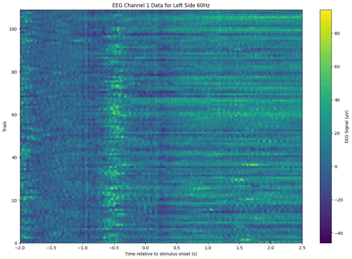
Visualise all channels separately
In [73]:
# Select data for a single trial from the 'left_side_60hz' condition
trial_data = eeg_data['left_side_60hz'][0, :, :]  # Select the first trial, all time points, all channels

# Calculate time vector based on the sampling rate and duration
sampling_rate = 2048  # in Hz
num_samples = trial_data.shape[0]
time_vector = np.linspace(-2, 2.5, num_samples)

# Create a figure with subplots
fig, axes = plt.subplots(8, 8, figsize=(20, 20), sharex=True, sharey=True)  # Adjust the grid size if needed

# Flatten the axes array for easy iteration
axes = axes.flatten()

for i in range(64):  # Assuming 64 channels
    ax = axes[i]
    ax.plot(time_vector, trial_data[:, i], color='black')
    ax.set_title(f'Ch {i+1}', fontsize=8)
    ax.set_xlim(time_vector[0], time_vector[-1])

# Set common labels
fig.text(0.5, 0.04, 'Time relative to stimulus onset (s)', ha='center', va='center')
fig.text(0.06, 0.5, 'EEG Signal (µV)', ha='center', va='center', rotation='vertical')

plt.suptitle('EEG Data Across 64 Channels for First Trial of Left Side 60Hz')
plt.tight_layout(rect=[0, 0.03, 1, 0.95])  # Adjust spacing to fit titles and labels
plt.show()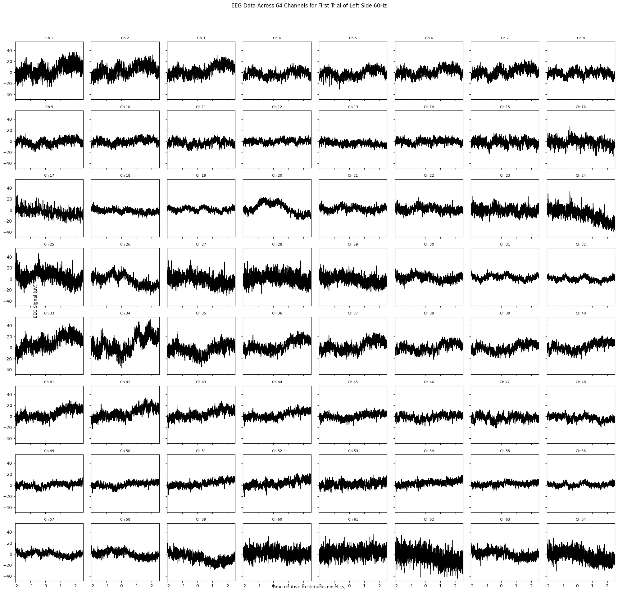
In [76]:
def plot_all_channels(eeg_data, condition, sampling_rate=2048):
    num_trials, num_samples, num_channels = eeg_data[condition].shape

    # Calculate time vector based on the sampling rate and duration
    time_vector = np.linspace(-2, 2.5, num_samples)

    # Set up the figure size
    plt.figure(figsize=(20, 30))

    # Loop over all channels
    for channel in range(num_channels):
        ax = plt.subplot(8, 8, channel + 1)
        channel_data = eeg_data[condition][:, :, channel]

        im = ax.imshow(channel_data, aspect='auto', extent=[time_vector[0], time_vector[-1], 0, num_trials], cmap='viridis')
        ax.set_title(f'Channel {channel + 1}')

    # Add colorbar
    plt.subplots_adjust(right=0.8)
    cbar_ax = plt.gcf().add_axes([0.85, 0.15, 0.05, 0.7])
    plt.colorbar(im, cax=cbar_ax, label='EEG Signal (µV)')

    # Add common labels
    plt.gcf().text(0.5, 0.04, 'Time relative to stimulus onset (s)', ha='center')
    plt.gcf().text(0.04, 0.5, 'Trials', va='center', rotation='vertical')

    plt.suptitle(f'EEG Data for {condition}', fontsize=16)
    plt.show()

# Visualise all channels for the left_side_60hz condition
plot_all_channels(eeg_data, 'left_side_60hz')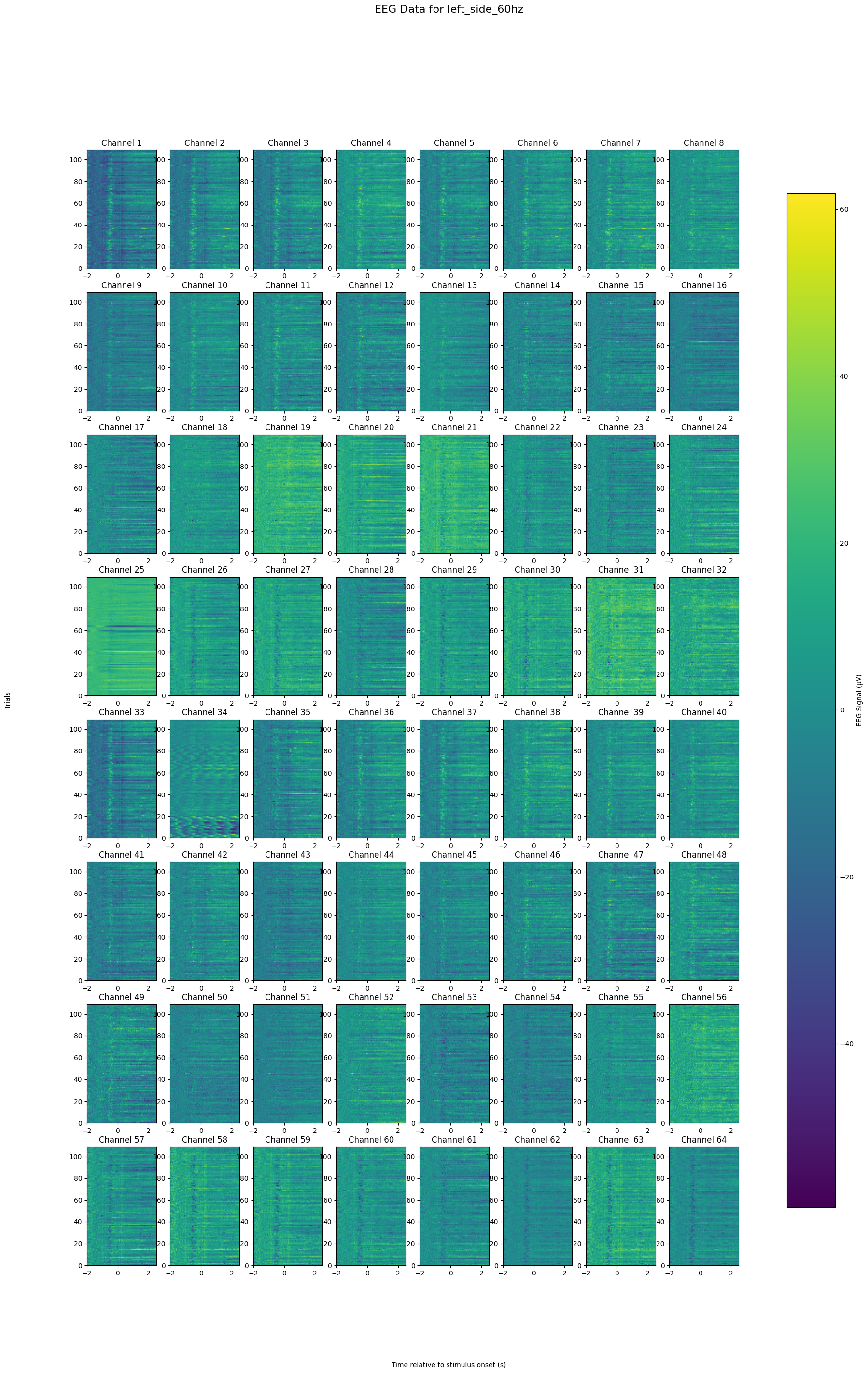
FFT one channel, one trial
In [94]:
def plot_fourier_spectrum(eeg_data, channel, trial, sampling_rate=2048):
    # Extract the signal for one channel and one trial
    signal = eeg_data[:, :, channel][trial, :]

    # Compute the Fast Fourier Transform (FFT)
    fft_signal = np.fft.fft(signal)

    # Compute the frequency bins
    freq_bins = np.fft.fftfreq(len(signal), d=1/sampling_rate)

    # Compute the magnitude of the FFT (for positive frequencies)
    magnitude = np.abs(fft_signal)[:len(signal)//2]
    frequencies = freq_bins[:len(signal)//2]

    # Plotting the spectrum
    plt.figure(figsize=(10, 5))
    plt.plot(frequencies, magnitude, color='blue')

    plt.title(f'Fourier Spectrum Analysis for Channel {channel+1}, Trial {trial+1}')
    plt.xlabel('Frequency (Hz)')
    plt.ylabel('Magnitude')
    plt.xlim(40, 80)  # Typically, EEG frequencies of interest are below 100 Hz
    plt.grid(True)

    plt.show()

# Example usage
# Assuming eeg_data is a NumPy array with the shape (trials, samples, channels)
# Let's use the first trial (index 0) and the first channel (index 0) as an example
plot_fourier_spectrum(eeg_data['left_side_64hz'], channel=1, trial=20)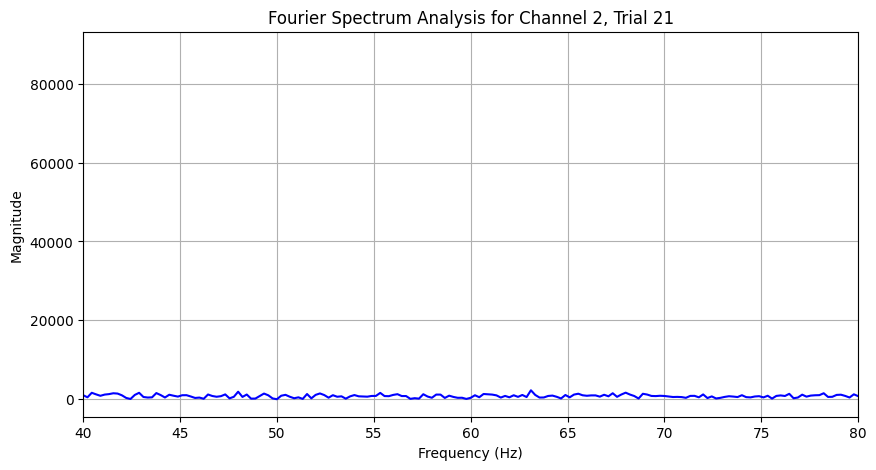
In [128]:
def plot_average_spectrum_all_channels(eeg_data, condition, sampling_rate=2048, min_frequency=40, max_frequency=80, start_time=None, end_time=None):
    num_trials, num_samples, num_channels = eeg_data[condition].shape
    time_step = 1 / sampling_rate
    frequencies = np.fft.fftfreq(num_samples, time_step)

    # Find indices for min and max frequency
    min_index = np.where(frequencies >= min_frequency)[0][0]
    max_index = np.where(frequencies >= max_frequency)[0][0]

    # Calculate the indices for the selected time frame
    start_index = int((start_time + 2) * sampling_rate) if start_time is not None else 0
    end_index   = int((  end_time + 2) * sampling_rate) if   end_time is not None else num_samples

    # Prepare the plot
    plt.figure(figsize=(12, 8))
    colors = cm.viridis(np.linspace(0, 1, num_channels))

    # Compute and plot the average spectrum for each channel
    for channel in range(num_channels):
        # Calculate the mean Fourier transform across all trials for the selected time frame
        fft_values = np.fft.fft(eeg_data[condition][:, start_index:end_index, channel], axis=1)
        mean_fft = np.mean(np.abs(fft_values), axis=0)

        # Plot the magnitude of the FFT
        plt.plot(frequencies[min_index:max_index], mean_fft[min_index:max_index], color=colors[channel], label=f'Channel {channel+1}')

    plt.title(f'Average Fourier Spectrum Across All Channels for {condition.split("_")[0].capitalize()} Side {condition.split("_")[-1][:-2]}Hz')
    plt.xlabel('Frequency (Hz)')
    plt.ylabel('Magnitude')
    plt.xlim(min_frequency, max_frequency)
    plt.legend(loc='upper right', ncol=2, fontsize='xx-small', title='Channels')
    plt.grid(True)
    plt.tight_layout()
    # Add vertical lines at 60 Hz and 64 Hz
    plt.axvline(x=60, color='red', linestyle='--', linewidth=1, label='60 Hz')
    plt.axvline(x=64, color='purple', linestyle='--', linewidth=1, label='64 Hz')
    plt.show()


plot_average_spectrum_all_channels(eeg_data, 'left_side_60hz', start_time=-2, end_time=0.5) # Before stimulus onset
plot_average_spectrum_all_channels(eeg_data, 'left_side_60hz', start_time=0.5, end_time=2.5) # After stimulus onset
plot_average_spectrum_all_channels(eeg_data, 'left_side_60hz') # Full time range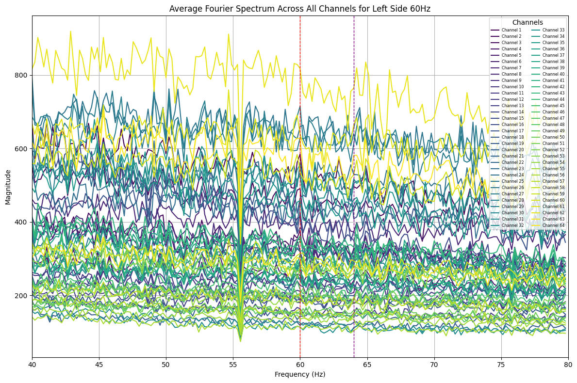
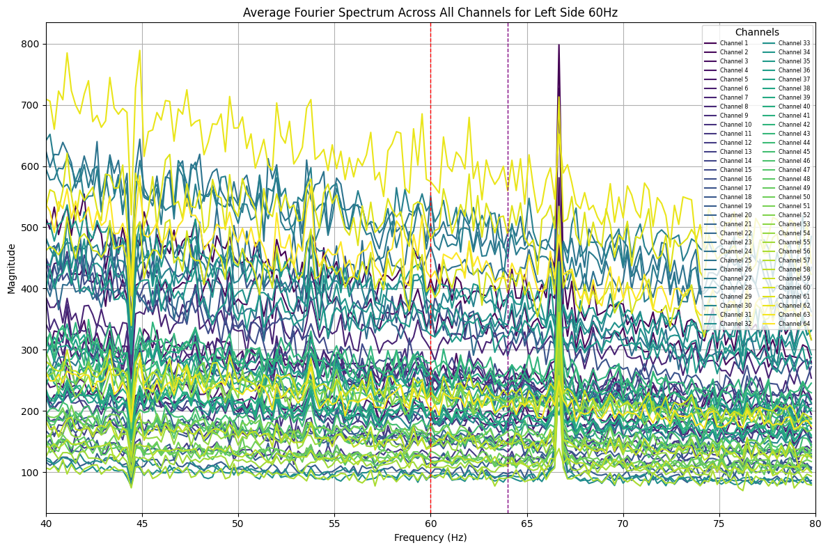
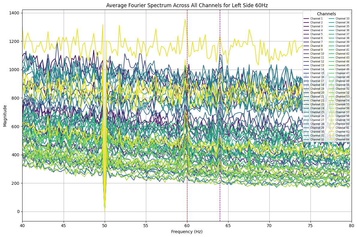
Analysis
Some peaks at 60Hz and 64Hz were visible in the full spectrum. Queer, now that I split the time ranges, some peaks have shown up at unexpected frequencies, this might be an aliasing problem :/. Will look into it later